CAIDA’s Annual 2024 Report
Friday, August 15th, 2025 by kcThe CAIDA annual report summarizes CAIDA’s activities for 2024 in the areas of research, infrastructure, data collection and analysis. The executive summary is excerpted below:
(more…)The CAIDA annual report summarizes CAIDA’s activities for 2024 in the areas of research, infrastructure, data collection and analysis. The executive summary is excerpted below:
(more…)We want to share important updates regarding our 100 GB anonymized passive trace initiative. The Los Angeles–San Jose link has been upgraded out of the range of this monitoring capability, so the monitor has transitioned to capture traffic traces on a different link.
Beginning in January 2025, we shifted our trace collection to a 100 GB link between Los Angeles and Dallas. This change opens up opportunities to study network dynamics across different infrastructures and geographies. For additional details, please visit https://catalog.caida.org/dataset/passive_2025_pcap_100g.
Based on a survey of 100 GB anonymized trace users, we have created and shared two complementary datasets to better serve the research community (1) a compilation of metadata statistics about the trace; and (2) a smaller (5-second) subset of data, which is less than 1GB of data compared to the full one-hour capture of about 600GB.
Distributed denial-of-service (DDoS) attacks are an ever-present phenomenon on the Internet. Over the years, many organizations and groups have undertaken efforts to reduce the feasibility and effectiveness of DDoS attacks, such as by disabling attack vectors (e.g., NTP’s get monlist), deploying source address validation (ingress & egress filtering), and enlisting law enforcement (booter takedowns). In addition, an industry of DDoS protection companies sells attack mitigation services. While these approaches have had some impact–who knows how dire the situation would be without such efforts?–DDoS remains a persistent threat.
A clear understanding and view of the DDoS landscape is the basis for developing and improving countermeasures. Our recent study comparatively evaluated long-term DDoS trends in academia and industry to better understand the current limitations. We focused on two classes of DDoS attacks: direct-path (DP) attacks and reflection-amplification (RA) attacks. In a direct-path attack, packets are sent directly to the target of the attack. One group of DP attacks establishes connections to abuse application layer protocols, while others use randomly spoofed source addresses. In a reflection-amplification attack, requests are spoofed to contain the source address of the attack target and sent to a reflective third party service (e.g., DNS), which then sends the replies to the victim.
Our study analyzed longitudinal DDoS trends across academia and industry. We collected 10 datasets from seven observatories listed in Table 1. Each observatory shared 4.5 years of weekly attack counts for our long-term trend analysis. The observatories from academia additionally shared raw DDoS event data, which enabled us to analyze the visibility of targets across observatories. We further collected and analyzed 24 DDoS threat reports from 22 companies for the year 2022. We published the detailed analysis as an artifact at https://ddoscovery.github.io.
| Observatory | Type | Coverage | DP Attack Trends | RA Attack Trends |
|---|---|---|---|---|
| UCSD NT | Network Telescope | 12M IPs | Increase 🔺 | (not applicable) |
| ORION NT | Network Telescope | 500k IPs | Increase 🔺 | (not applicable) |
| Netscout Atlas | On-path Network | Proprietary | Increase 🔺 | Increase 🔺 |
| Akamai Prolexic | On-path Network | Proprietary | Neutral 🔴 | Neutral 🔴 |
| IXP Blackholing | On-path Network | Proprietary | Increase 🔺 | Decrease 🔻 |
| AmpPot | Honeypot | ~30 IPs | (not applicable) | Neutral 🔴 |
| Hopscotch | Honeypot | 65 IPs | (not applicable) | Decrease 🔻 |
| Industry Reports | PDF/website/etc. | 22 Companies | Increase 🔺 | Increase 🔺 and Decrease 🔻 |
Our analysis of attack trends revealed that even observatories that agree on long-term trends (Table 1) exhibit many differences in short-term patterns, reflecting different views of the DDoS landscape. For the analysis, we normalized the weekly attack counts to the median of the first 15 weeks. We plot the exponentially weighted moving average (EWMA) with a 12-week window and linear regressions starting in 2019 and ending in 2022.
Both network telescopes (Fig. 1) observed an increase in attacks during the measurement period. They repeatedly saw short peaks that at least tripled attack counts, but did not coincide across both observatories. ORION saw its largest peaks in 2022Q1 and Q2, with smaller peaks in 2019Q2 and mid-2021. In contrast, UCSD saw its largest peak in 2023, with small peaks in each year. While ORION observed a decline in 2023 compared to 2022, UCSD trends remained positive.
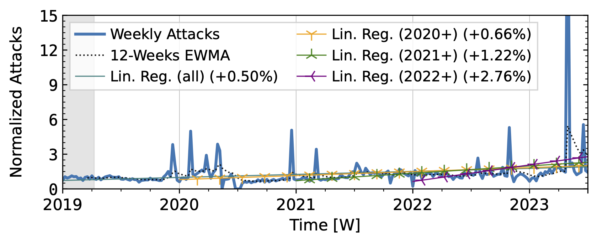
Figure 1 a): The long-term trends of (randomly-spoofed) direct-path attacks observed by UCSD NT.
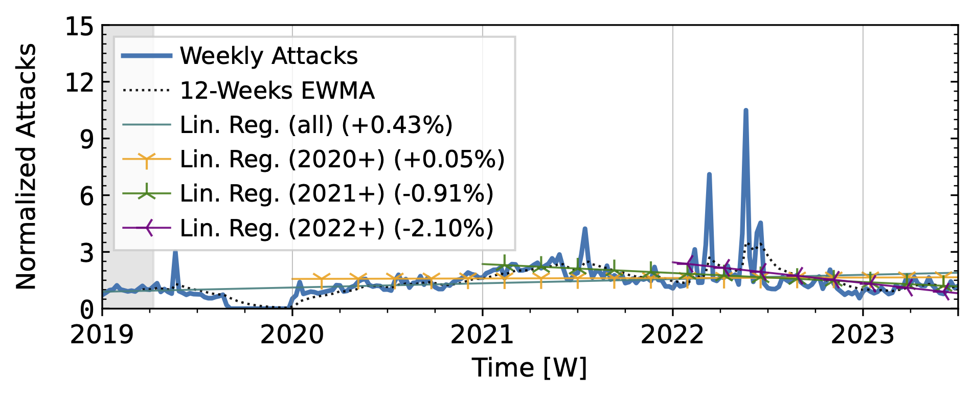
Figure 1 b): The long-term trends of (randomly-spoofed) direct-path attacks observed by ORION NT
The time series from one of our industry observatories (Figure 2) did not show large peaks. Netscout Atlas (Fig. 2a) experienced stable growth, except in 2021. Akamai Prolexic (Fig. 2b) fluctuated around its baseline with a slight decrease in attacks overall. Both companies likely have stable customer bases and are less affected by sudden bursts in attacks. Both companies saw a rise in attacks in 2020, followed by a decline in 2021. Netscout saw a rise throughout 2022, while Akamai saw peaks in 2022 but no persistent increase. Both companies detected a rise in attacks in 2023.
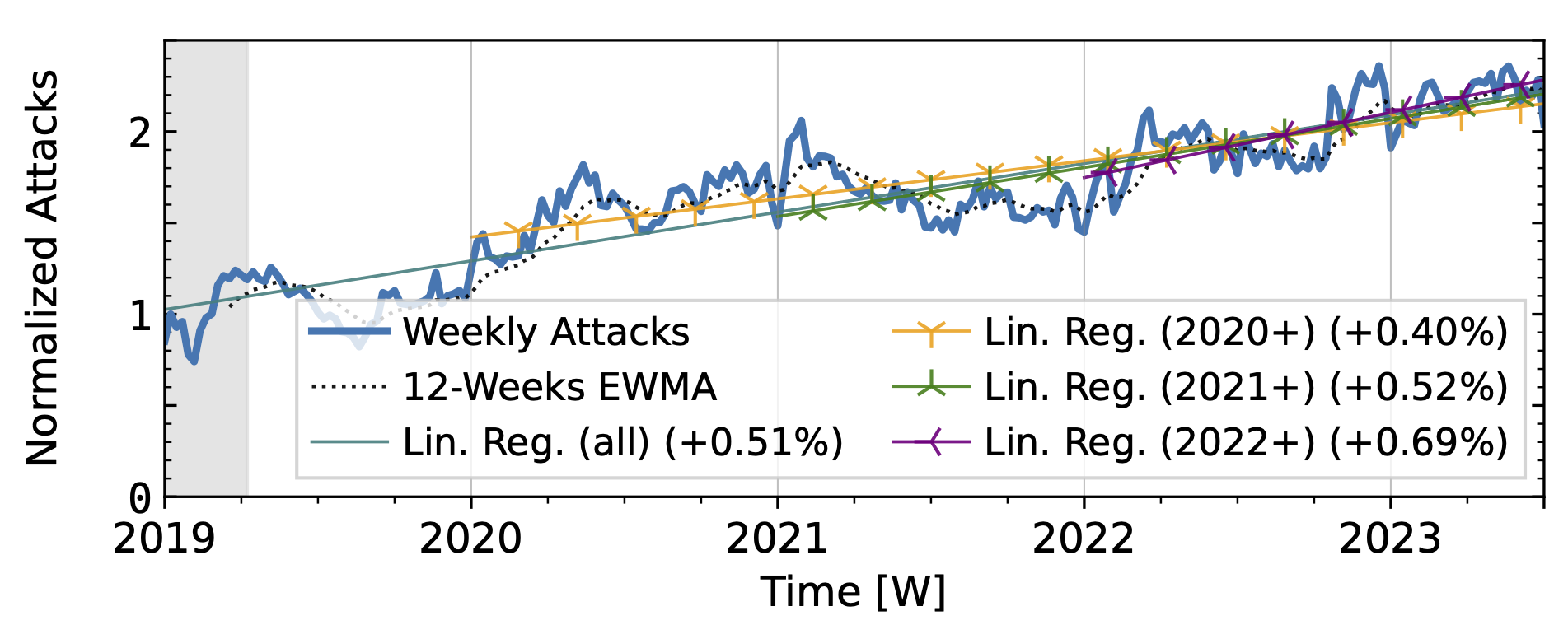
Figure 2 a): Long-term trends of direct-path attacks observed by Netcout Atlas.
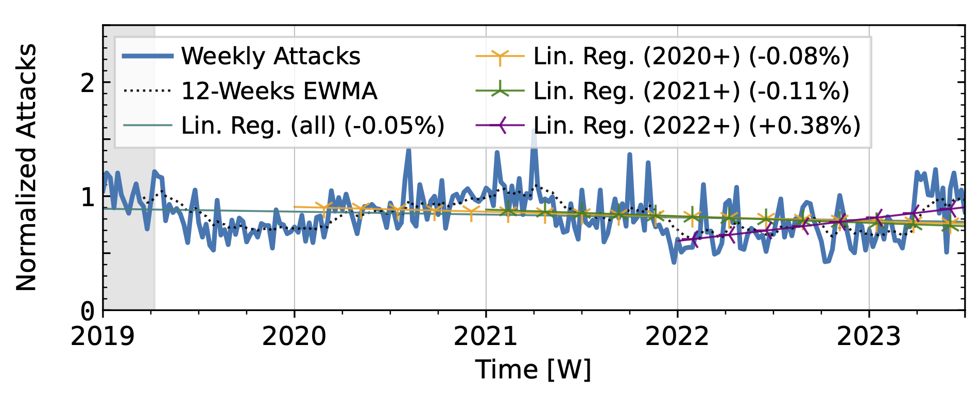
Figure 2 b): Long-term trends of direct-path attacks observed by Akamai Prolexic.
The honeypots in our study (Fig. 3) showed a significant increase in attacks in 2020 after a decline in 2019Q4. Hopscotch recorded most attacks early in 2020, while AmpPot saw its highest peaks later, coinciding with a decline in attack counts at Hopscotch. Both HPs detected a continued decline in 2021, aligning with industry efforts to deploy SAV (see discussion in the paper, Section 2.3). While both time series shared a peak in mid-2022, the peak was much more pronounced in the Hopscotch data.
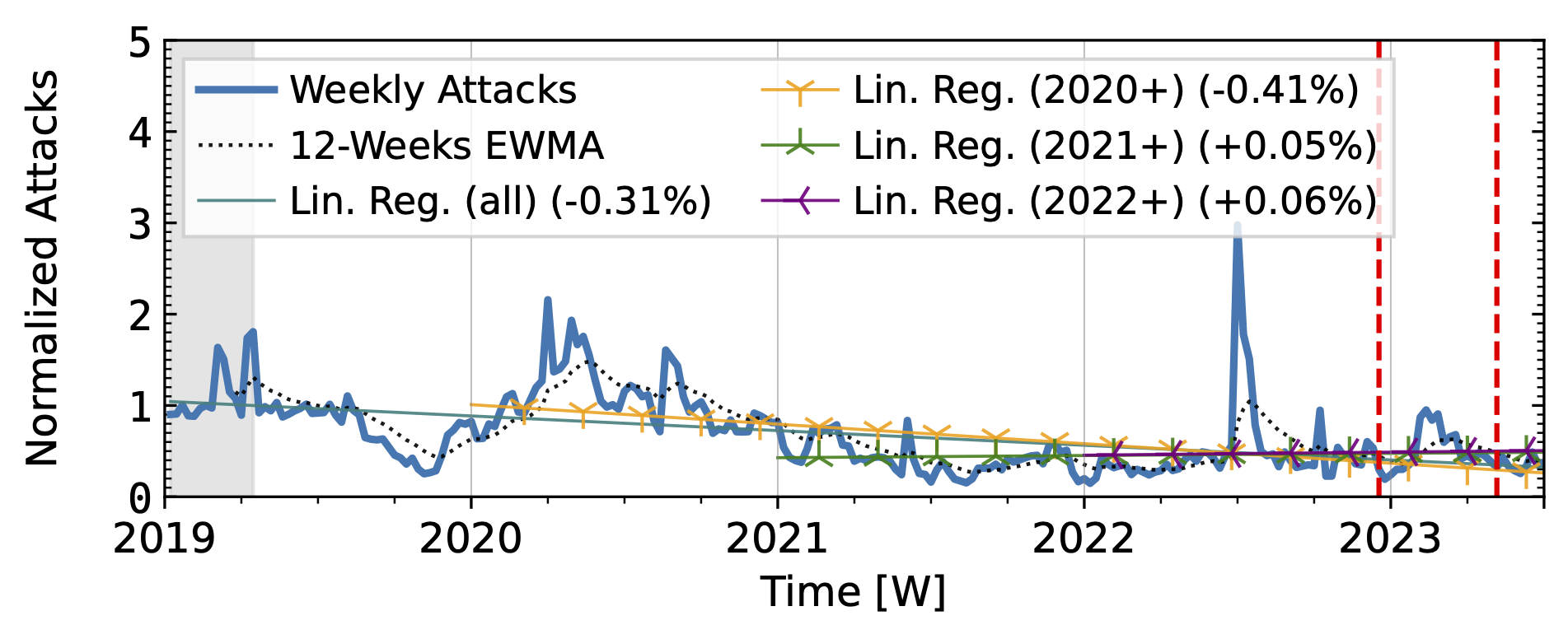
Figure 3 a): Long-term trends of reflection-amplification attacks observed by Hopscotch. The red dashed lines mark DDoS takedown efforts by law enforcement.
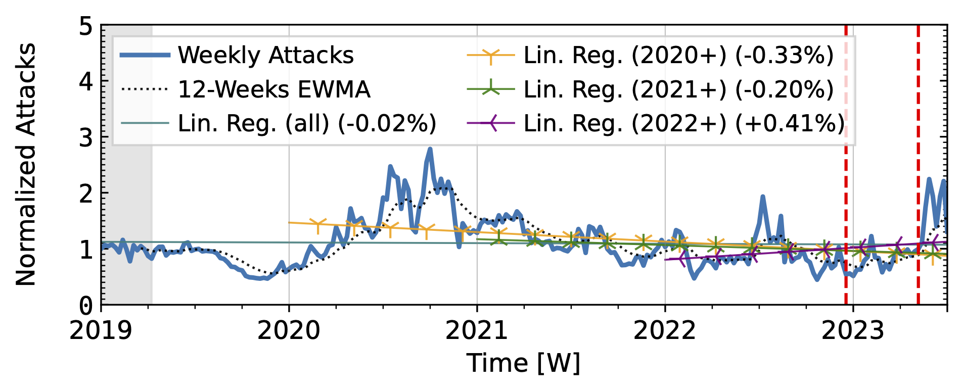
Figure 3 b): Long-term trends of reflection-amplification attacks observed by AmpPot. The red dashed lines mark DDoS takedown efforts by law enforcement.
Akamai Prolexic (Fig. 4 a) experienced only small variations in attacks until 2020Q3 before they surged above 2x its baseline in 2021Q1. This peak coincided with a peak in the IXP time series (Fig. 4 b). However, the IXP already saw a steep rise in attacks starting in 2019Q4, with peaks in 2021Q1 and Q2. Both time series declined until the end of 2022, with more pronounced peaks in the Akamai time series. They both detected an increase in attacks in 2023 but had a neutral to negative trend overall.
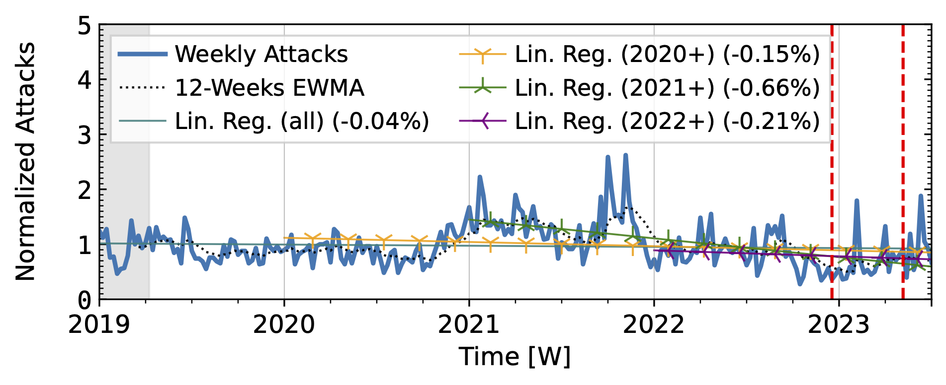
Figure 4 a): Long-term trends of reflection-amplification attacks observed by Akamai Prolexic. The red dashed lines mark DDoS takedown efforts by law enforcement.
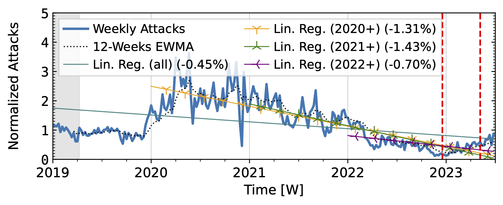
Figure 4 b): Long-term trends of reflection-amplification attacks observed in IXP Blackholing. The red dashed lines mark DDoS takedown efforts by law enforcement.
Booter takedowns by law enforcement. We marked known booter takedowns by law enforcement with red dashed lines in Figures 3 and 4. Booters offer DDoS-as-a-service usually relying on reflection-amplification attacks. The first takedown in late 2022Q4 led to immediate, small valleys in all graphs. In contrast, the 2023Q2 takedown did not affect the AmpPot time series (Fig. 3 b). Instead, attack counts increased. While we do not know how trends would have evolved without interference, the impact on DDoS trends appears limited in our time series.
We investigated the cause of these differences by comparing DDoS targets across observatories (Section 7 in our paper). The analysis revealed that our four observatories from academia saw a substantial share of targets that were not seen by the other three. While the overlap among observatories of the same type, i.e., either honeypots or network telescopes, was considerable, each observatory provided a unique view into the DDoS attack landscape. This highlights the limitations of individual datasets and the root cause of different views of the DDoS landscape. Overlap between observatories from academia and industry was similarly limited. Thus, cooperation with industry partners is a valuable–and potentially necessary–source for improved visibility.
Our analysis of 10 longitudinal datasets from 7 observatories revealed the limited view that researchers have as a basis for DDoS research. Without an accurate view we can neither accurately plan actions nor evaluate their outcome.
Advice for researchers: DDoS research tries to make global inferences based on local views. Accepting and acknowledging the limitations of available datasets is important for accurate interpretation and comparison. When possible, researchers should analyze multiple datasets, which generally requires collaboration with operators. In parallel, stakeholders across academia and industry need to converge on specific frameworks for data sharing to facilitate comparison. Unexplored details include the definition of incidents and their impact, data formats to accommodate comparisons, disclosure control technologies, and access policies to allow rigorous independent analyses.
Advice for threat-intelligence companies: Collaborate with researchers. Gathering reliable data on DDoS attacks is challenging. Getting additional data from different vantage points–especially those that academia usually has no access to–is invaluable for researchers. We found that many DDoS reports are only available after providing email addresses and are not archived for long-term access. Lowering the effort to read reports and archiving historical reports increases visibility and perspective on trends over time. Since language is often not consistent across companies and since vantage points and methodologies differ, comparisons to previous reports from the same company are especially relevant to analyze long-term changes in the DDoS landscape.
Advice for operators: Spoofing is an integral mechanism abused in many DDoS attacks, including all reflection-amplification attacks and a significant subset of direct-path attacks. Source address validation (SAV) is an effective tool to stop these attacks. Supporting ongoing research and extending measurement systems to quantify the deployment of SAV and reveal persistent sources of spoofed packets is a challenging but worthwhile undertaking.
Let’s collaborate to achieve a comprehensive view of DDoS!
Paper Reference: Raphael Hiesgen, Marcin Nawrocki, Marinho Barcellos, Daniel Kopp, Oliver Hohlfeld, Echo Chan, Roland Dobbins, Christian Doerr, Christian Rossow, Daniel R. Thomas, Mattijs Jonker, Ricky Mok, Xiapu Luo, John Kristoff, Thomas C. Schmidt, Matthias Wählisch, KC Claffy, The Age of DDoScovery: An Empirical Comparison of Industry and Academic DDoS Assessments, In: Proc. of ACM Internet Measurement Conference (IMC), p. 259–279, ACM : New York, 2024. https://doi.org/10.1145/3646547.3688451
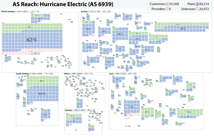
The AS Reach Visualization provides a geographic breakdown of the number of ASes reachable through an AS’s customer, peers, providers, or an unknown neighbor. The interactive interface to the visualization can be found at https://www.caida.org/catalog/media/visualizations/as-reach/
Independent networks (Autonomous Systems, or ASes) engage in typically voluntary bilateral interconnection (“peering”) agreements to provide reachability to each other for some subset of the Internet. The implementation of these agreements introduces a non-trivial set of constraints regarding paths over which Internet traffic can flow, with implications for network operations, research, and evolution. Realistic models of Internet topology, routing, workload, and performance
must account for the underlying economic dynamics.
Although these business agreements between ISPs can be complicated, the original model introduced by Gao (On inferring autonomous system relationships in the Internet), abstracts business relationships into the following three most common types:
An AS’s Reach is defined as the set of ASes the target AS can reach through its customers, peers, providers, or unknown. The Customer Reach is the set of ASes reachable through the AS’s customers. The Peer Reach is the set of ASes that are not in the Customer Reach, but reachable through the AS’s peers. The Provider Reach is the set of ASes not in the Customer or Peer Reach, but reachable through the AS’s provider. The Unknown Reach is the set of ASes not in the Customer, Peer, or Provider Reach. More details at https://www.caida.org/catalog/media/visualizations/as-reach/
The CAIDA annual report (quite a bit later than usual this year due to an unprecedented level of activity in 2024 which we will report on earlier next year!) summarizes CAIDA’s activities for 2023 in the areas of research, infrastructure, data collection and analysis. The executive summary is excerpted below:
(more…)
This is the third in a series of essays (two earlier blog posts [1, 2]) about CAIDA’s new effort to reduce the barrier to performing a variety of Internet measurements.
We were recently asked about running Trufflehunter, which infers the usage properties of rare domain names on the Internet by cache snooping public recursive resolvers, on Ark. The basic idea of Trufflehunter is to provide a lower bound of the use of a domain name by sampling caches of large recursive resolvers. One component of Trufflehunter is to identify the anycast instances that would answer a given vantage point’s DNS queries. Trufflehunter uses a series of TXT queries to obtain the anycast instance of a given public recursive resolver, and considers four large public recursive resolvers: Cloudflare (1.1.1.1), Google (8.8.8.8), Quad9 (9.9.9.9), and OpenDNS (208.67.220.220). The original paper describes the queries in section 4.1, which we summarize below, highlighting the interesting parts of each response with blue color.
Cloudflare returns an airport code representing the anycast deployment location used by the VP:
$ host -c ch -t txt id.server 1.1.1.1

id.server descriptive text "AKL"
Google returns an IP address representing the anycast deployment used by the VP, which can be mapped to an anycast deployment location with a second query:
$ host -t txt o-o.myaddr.l.google.com 8.8.8.8

o-o.myaddr.l.google.com descriptive text "172.253.218.133"

o-o.myaddr.l.google.com descriptive text "edns0-client-subnet <redacted>/24"
$ host -t txt locations.publicdns.goog

locations.publicdns.goog descriptive text "34.64.0.0/24 icn " ... "172.253.218.128/26 syd " "172.253.218.192/26 cbf " ...
Quad9 returns the hostname representing the resolver that provides the answer:
$ host -c ch -t txt id.server 9.9.9.9

id.server descriptive text "res100.akl.rrdns.pch.net"
and finally, OpenDNS returns a bunch of information in a debugging query, which includes the server that handles the query:
$ host -t txt debug.opendns.com 208.67.220.220

debug.opendns.com descriptive text "server r2004.syd"

debug.opendns.com descriptive text "flags 20040020 0 70 400180000000000000000007950800000000000000"

debug.opendns.com descriptive text "originid 0"

debug.opendns.com descriptive text "orgflags 2000000"

debug.opendns.com descriptive text "actype 0"

debug.opendns.com descriptive text "source <redacted>:42845"
Each of these queries requires a slightly different approach to extract the location of the anycast instance. Our suggestion is for experimenters to use our newly created python library, which provides programmatic access to measurement capabilities of Ark VPs (described in two earlier blog posts [1, 2]). The code for querying the recursive resolvers from all VPs is straight forward, and is shown below. First, on lines 15-27, we get the Google mapping, so that we can translate the address returned to an anycast location. This query requires TCP to complete, as the entry is larger than can fit in a UDP payload (the response is 9332 bytes at the time of writing this blog). This query is synchronous (we wait for the answer before continuing, because the google queries that follow depend on the mapping) and is issued using a randomly selected Ark VP. Then, on lines 29-38, we issue the four queries to each of the anycasted recursive resolvers from each VP. These queries are asynchronous; we receive the answers as each Ark VP obtains a response. On lines 40-82, we process the responses, storing the results in a multi-dimensional python dictionary, which associates each Ark VPs with their anycast recursive resolver location, as well as the RTT between asking the query and obtaining the response. Finally, on lines 84-96, we dump the results out in a nicely formatted table that allows us to spot interesting patterns.
01 import argparse

02 import datetime

03 import ipaddress

04 import random

05 import re

06 from scamper import ScamperCtrl

07

08 def _main():

09   parser = argparse.ArgumentParser(description='get public recursive locs')

10   parser.add_argument('sockets')

11   args = parser.parse_args()

12

13   ctrl = ScamperCtrl(remote_dir=args.sockets)

14

15   # pick an ark VP at random to issue the query that gets the mapping

16   # of google recursive IP to location

17   goog_nets = {}

18   obj = ctrl.do_dns('locations.publicdns.goog',

19     inst=random.choice(ctrl.instances()),

20     qtype='txt', tcp=True, sync=True)

21   if obj is None or len(obj.ans_txts()) == 0:

22     print("could not get google mapping")

23     return

24   for rr in obj.ans_txts():

25     for txt in rr.txt:

26       net, loc = txt.split()

27       goog_nets[ipaddress.ip_network(net)] = loc

28

29   # issue the magic queries to get the instance that answers the query

30   for inst in ctrl.instances():

31     ctrl.do_dns('o-o.myaddr.l.google.com', server='8.8.8.8', qtype='txt',

32       attempts=2, wait_timeout=2, inst=inst)

33     ctrl.do_dns('id.server', server='1.1.1.1', qclass='ch', qtype='txt',

34       attempts=2, wait_timeout=2, inst=inst)

35     ctrl.do_dns('id.server', server='9.9.9.9', qclass='ch', qtype='txt',

36       attempts=2, wait_timeout=2, inst=inst)

37     ctrl.do_dns('debug.opendns.com', server='208.67.220.220', qtype='txt',

38       attempts=2, wait_timeout=2, inst=inst)

39

40   # collect the data

41   data = {}

42   for obj in ctrl.responses(timeout=datetime.timedelta(seconds=10)):

43     vp = obj.inst.name

44     if vp not in data:

45       data[vp] = {}

46     dst = str(obj.dst)

47     if dst in data[vp]:

48       continue

49     data[vp][dst] = {}

50     data[vp][dst]['rtt'] = obj.rtt

51

52     for rr in obj.ans_txts():

53       for txt in rr.txt:

54         if dst == '8.8.8.8':

55           # google reports an IPv4 address that represents

56           # the site that answers the query. we then map

57           # that address to a location using the mapping

58           # returned by the locations TCP query.

59           try:

60             addr = ipaddress.ip_address(txt)

61           except ValueError:

62             continue

63           for net, loc in goog_nets.items():

64             if addr in net:

65               data[vp][dst]['loc'] = loc

66               break

67         elif dst == '1.1.1.1':

68           # Cloudflare replies with a single TXT record

69           # containing an airport code

70           data[vp][dst]['loc'] = txt

71         elif dst == '9.9.9.9':

72           # Quad9 reports a hostname with an embedded

73           # airport code.

74           match = re.search("\\.(.+?)\\.rrdns\\.pch\\.net", txt)

75           if match:

76             data[vp][dst]['loc'] = match.group(1)

77         elif dst == '208.67.220.220':

78           # opendns reports multiple TXT records; we want the one

79           # that looks like "server r2005.syd"

80           match = re.search("^server .+\\.(.+?)$", txt)

81           if match:

82             data[vp][dst]['loc'] = match.group(1)

83

84   # format the output

85   print("{:15} {:>13} {:>13} {:>13} {:>13}".format(

86     "# vp", "google", "couldflare", "quad9", "opendns"))

87   for vp, recs in sorted(data.items()):

88     line = f"{vp:15}"

89     for rec in ('8.8.8.8', '1.1.1.1', '9.9.9.9', '208.67.220.220'):

90       cell = ""

91       if 'loc' in recs[rec]:

92         rtt = recs[rec]['rtt']

93         loc = recs[rec]['loc']

94         cell = f"{loc} {rtt.total_seconds()*1000:5.1f}"

95       line += f" {cell:>13}"

96     print(line)

97

98 if __name__ == "__main__":

99     _main()
The code runs quickly — no longer than 10 seconds (if one of the VPs is slow to report back), illustrating the capabilities of the Ark platform.
The output of running this program is shown below. We have highlighted cells where the RTT was at least 50ms larger than the minimum RTT to any of the large recursive resolvers for the given VP. These cells identify low-hanging fruit for operators, who could examine BGP routing policies with the goal of selecting better alternative paths.
# vp             google   couldflare         quad9      opendns

abz-uk.ark    lhr  24.4    LHR  16.5     lhr  16.9    lon  16.4

abz2-uk.ark   lhr  23.4    MAN   8.7     man   8.4   man1   8.5

acc-gh.ark    jnb 246.7    JNB 167.3     acc   0.5   cpt1 236.6

adl-au.ark    mel  28.1    ADL   5.5     syd  22.6   mel1  14.0

aep-ar.ark    scl  29.4    EZE   8.0   qaep2   4.6   sao1  34.0

aep2-ar.ark   scl  38.2    EZE   6.6   qaep2   5.7   sao1  42.5

akl-nz.ark    syd   26.9    AKL   2.6    akl2   4.0    syd  26.1

akl2-nz.ark   syd   29.2    AKL   4.9    akl2   4.0    syd  26.9

ams-gc.ark    grq   5.0    FRA   6.3     ams   0.8    ams   1.1

ams3-nl.ark   grq   6.0    AMS   2.1     ams   1.3    ams   1.9

ams5-nl.ark   grq   5.1    AMS   1.2     ams   1.9    ams   1.7

ams7-nl.ark   grq    6.0    AMS   2.4     ams   1.8    ams   2.3

ams8-nl.ark   grq  14.8    AMS  11.5     fra  17.7    ams  11.8

arn-se.ark    lpp   9.7    ARN   2.0     arn   0.8   cph1  10.5

asu-py.ark    scl  55.4    EZE  22.6     asu   0.8   sao1  57.0

atl2-us.ark   atl   9.8    DFW  23.6   qiad3  20.5   atl1   4.6

atl3-us.ark   atl  22.7    ATL  13.1     atl  17.0   atl1  19.7

aus-us.ark    dfw  80.7    DFW  56.6     dfw  46.6    dfw  17.6

avv-au.ark    mel 142.3    MEL   9.4     syd  22.6   mel1   8.5

bcn-es.ark    mad  38.0    BCN  13.3     bcn   0.5   mad1   9.8

bdl-us.ark    iad  13.3    EWR   5.0     lga   4.9    ash  10.6

bed-us.ark    iad  30.6    BOS  15.2     bos  13.5   bos1  19.8

beg-rs.ark    mil  62.5    BEG   1.2     beg   0.7   otp1  12.9

bfi-us.ark    dls  11.7    SEA   3.8   xsjc1  96.9    sea  10.5

bjl-gm.ark    bru  87.5    CDG  71.1     bjl   6.7   cdg1  73.4

bna-us.ark    atl  11.4    BNA   9.0     atl   9.5   atl1   9.3

bna2-us.ark   cbf  25.5    ORD  19.7     ord  12.8    chi  12.8

bos6-us.ark   iad  17.6    BOS   5.6   qiad3  15.5   bos1   5.7

bre-de.ark    grq  21.4    TXL  23.1     ber  17.2    ams  23.7

btr-us.ark    dfw  20.3    ORD  29.5     dfw  13.2    dfw  11.4

bwi2-us.ark   iad  12.7    IAD   4.4   qiad3   3.6   rst1   3.1

cdg-fr.ark    mil  24.9    MRS   1.5     mrs   1.0   mrs1  11.6

cdg3-fr.ark   bru   8.5    CDG   3.9     ams  13.7   cdg1   5.5

cgs-us.ark    iad   4.5    EWR   7.9     iad   2.2    ash   2.1

cjj-kr.ark    hkg  63.4                qhnd2  70.7    hkg  47.3

cld4-us.ark   lax  22.7    LAX  15.7     bur 104.1    lax  14.3

cld5-us.ark   lax  52.6    LAX  20.7     bur 103.1    lax  21.9

cld6-us.ark   lax  14.5    LAX   5.2   qlax1   7.0    lax   6.0

cos-us.ark    cbf  22.9    DEN   7.3     ord  36.0   den1  12.6

dar-tz.ark    jnb 224.6    NBO  14.0     dar   1.0    jnb  51.1

dar2-tz.ark   jnb 223.0    DAR   0.9     dar   0.9    jnb  48.0

dmk-th.ark    sin  32.2    SIN  28.0     bkk   2.4   nrt2  95.0

dtw2-us.ark   cbf  18.1    DTW   4.6     dtw   4.2    chi  10.7

dub-ie.ark    lhr  18.9    DUB   1.2     dub   0.7   dub1   0.7

dub2-ie.ark   lhr  18.7    DUB   1.8     dub   1.1   dub1   1.2

dub3-ie.ark   lhr  35.5    ZRH  45.6     dub  16.9   dub1  11.6

ens-nl.ark    grq   9.3    AMS   5.2     ams   4.0    ams   4.9

eug-us.ark    dls  15.7    SJC  18.3     sea   6.5    sea   6.5

fra-gc.ark    fra   9.1    FRA   1.1     fra   1.1    fra   1.1

gig-br.ark    gru 125.2    GIG   2.2   qrio1   1.4   rio1   1.1

gva-ch.ark                 ZRH   5.3     gva   1.0    fra  10.8

gye-ec.ark    chs 128.7    MIA  66.8   quio2  10.7    mia  77.1

ham-de.ark    grq  19.7    HAM   8.5     ber  11.0    fra  17.7

her2-gr.ark   mil  64.9                  ath   7.5   mil1  32.6

hkg4-cn.ark   tpe  13.6    HKG   1.0   qhkg3   4.9    hkg   9.5

hkg5-cn.ark   hkg  16.3    HKG   2.6   qhkg3   3.9    hkg   3.6

hlz2-nz.ark   syd  40.9    AKL  16.9     akl  13.8    syd  38.2

hnd-jp.ark    nrt   6.5    NRT   3.4   qhnd2  80.3    nrt   3.6

hnl-us.ark    dls  82.3    HNL   1.1     sea  75.2    sea  75.3

iev-ua.ark    waw  45.5    FRA  29.8   qwaw2  14.3   wrw1  14.9

igx2-us.ark   iad  16.1    EWR  16.9   qiad3  11.5   atl1  11.8

ind-us.ark    atl  25.1    IND   1.1     ord   8.5   atl1  11.0

ixc-in.ark    del  78.8    DEL   0.8   qsin1   0.7   mum2   0.7

jfk-us.ark    iad   9.6    EWR   1.5     lga   0.6    nyc   1.0

kgl-rw.ark    jnb 231.6    NBO  15.0     kgl   3.3    jnb  73.6

ktm-np.ark    del  98.6    DEL  30.4     ktm   7.6   mum1  94.4

las-us.ark    lax  15.5    LAX   8.4     pao  15.9    lax   8.2

lax3-us.ark   lax  10.5    LAX   3.0     bur   2.0    lax   2.0

lcy2-uk.ark   lhr  11.5    MAN   7.4     lhr  11.2    lon   2.2

lej-de.ark    fra  21.2    FRA   9.7     fra  12.5    fra   9.6

lex-us.ark    iad  17.9    IAD  15.7     iad  17.3   atl1  25.9

lgw-uk.ark    lhr  31.3    LHR  24.2     lhr  24.6    lon  23.6

lhe2-pk.ark   dia 195.0    KHI  35.0   qsin4 113.1    sin 130.6

lis-pt.ark    mad  33.0    LIS   4.5     lis   3.9   mad1  18.0

lke2-us.ark   dls  21.7    SEA  21.4     sea  15.1    sea  11.7

lun-zm.ark    jnb 189.9    JNB  32.2     jnb  23.3    jnb  23.3

lwc-us.ark    tul  18.0    MCI   1.4   xsjc1 106.3    dfw  10.4

lwc2-us.ark   dfw  24.4    DFW  15.7   qlax1  46.9    dfw  16.5

mdw-us.ark    cbf  25.7    ORD   7.0     ord   3.4    chi   4.4

med2-co.ark   mrn  96.4    MIA  50.7   qbog1  22.7    mia  48.9

mhg-de.ark    fra  30.7    FRA  19.1     fra  21.4    fra  18.4

mia-gc.ark    mrn  19.7    MIA   1.1     mia   1.0    mia   0.6

mnl-ph.ark    hkg  87.9    MNL   1.8   qsin1  50.8    hkg  75.8

mnz-us.ark    iad  13.4    IAD   5.8   qiad3   5.2   rst1   4.0

mru-mu.ark    jnb 206.1    JNB  43.1     mru   1.0    jnb  43.3

msy-us.ark    dfw  34.4    DFW  21.9   qlax1  55.2    dfw  23.0

mty-mx.ark    tul  44.1    MFE   4.5   qiad3  39.6    dfw  16.7

muc-de.ark    fra  30.3    FRA   9.1     fra   8.8    fra   8.9

muc3-de.ark   zrh  25.9    MUC   6.1     fra  11.0    fra  12.2

nap2-it.ark   mil  37.8    MXP  19.8     fra  38.0   mil1  15.2

nbo-ke.ark    jnb 220.5    NBO   2.4     nbo   2.2    jnb  60.7

nic-cy.ark    mil  61.3    LCA   1.0     mrs  35.2   mrs1  35.4

nrn-nl.ark    grq   8.6    AMS   5.5     ams   2.9    ams   3.1

nrt-jp.ark    nrt   4.8    NRT   1.2     hkg 101.9   nrt2   1.0

nrt3-jp.ark   nrt   6.5    NRT   3.5     pao 101.7   nrt2   3.5

oak5-us.ark   lax  19.3    SJC   5.9    sjc0   4.4    pao   4.4

okc-us.ark    dfw   9.6    MCI   9.6     dal   8.2    dfw   7.3

ord-us.ark    cbf  13.0    ORD   2.9     iad  19.0    chi   1.6

ory4-fr.ark   bru   6.5    CDG   2.0     cdg   1.4   cdg1   1.7

ory6-fr.ark   bru   6.4    LHR   8.8     lhr   8.4    lon   8.6

ory7-fr.ark   bru   7.7    CDG   4.0     cdg   5.0   cdg1   4.0

ory8-fr.ark   bru   6.3    CDG   2.0     lhr  25.7    lon   9.4

osl-no.ark    lpp  46.5    OSL   0.9     osl  25.8   sto1   9.0

pbh2-bt.ark   bom 105.2    MAA  92.0     pbh   1.8    sin  91.7

per-au.ark    syd  48.9    PER   2.0     per   1.2    syd  45.3

per2-au.ark   syd 140.0    PER   2.5     per   1.5    syd  44.9

phl-us.ark    iad  15.9                  iad  14.0   rst1  15.9

pna-es.ark    mad  33.9    BCN  13.5     bcn  13.3   mad1  19.3

prg-cz.ark    fra  16.9    PRG   1.1   qbts1   5.9   prg1   0.6

prg2-cz.ark   fra  29.8    PRG   1.7   qfra3  14.0   prg1   1.5

pry-za.ark    jnb 167.3    JNB   1.2     jnb   0.6   cpt1  18.4

puw-ru.ark    lpp  18.2    DME   1.5     beg  67.1    fra  34.3

pvu-us.ark    lax  25.2    SLC   3.8     slc   2.7    sea  18.4

rdu-us.ark    iad   9.5    IAD   8.1     iad   7.7    ash   8.6

rdu2-us.ark   iad  11.3    IAD   8.1     iad   8.5    ash   8.6

rdu3-us.ark   iad  27.5    IAD  18.6     iad  18.4   atl1  23.8

rkv-is.ark    lhr  49.0    KEF   2.0     kef   0.8   dub1  23.0

san-us.ark    lax  10.4    LAX   4.7     bur  87.2    lax   3.1

san2-us.ark   lax  39.0    LAX   6.5   qlax1   7.5    lax   5.6

san4-us.ark   lax  26.6    LAX  20.2     bur 106.8    lax  17.3

sao-br.ark    gru 117.3    GRU   2.5   qgru1   1.3   rio1   9.6

scq-es.ark    mad  31.7    MAD  11.0     mad  10.8   mad1  11.3

sea3-us.ark   dls  10.1    SEA   3.9     pao  24.6    sea   3.0

sin-gc.ark    sin   4.0    SIN   1.5   qsin1  93.5    sin   1.1

sin-sg.ark    sin   3.2    SIN   2.3   qsin1  12.2    sin   0.7

sjc2-us.ark   lax  15.2    SJC   1.4    sjc0   0.5    pao   2.1

sjj-ba.ark    waw  71.1    BUD  57.5     vie 213.3   mil1  89.4

sjo-cr.ark    chs  63.0    SJO   2.2     mia  51.8    mia  78.6

snn-ie.ark    lhr  20.4    DUB   4.4     dub   3.9   dub1   3.9

sql-us.ark    lax  19.6    SJC   2.2     pao   1.2    pao   0.9

stx-vi.ark    chs  38.3    MIA  26.4     mia  25.5    mia  25.1

svo2-ru.ark   lpp  22.4    DME   5.8     fra  41.1    fra  38.2

swu-kr.ark    hkg  77.6    ICN   6.5   qsin1  76.9   nrt2  38.5

syd3-au.ark   syd   4.8    SYD   0.9     syd   1.0    syd   0.5

tij-mx.ark    lax  15.8    LAX   6.6   qlax1   6.6    lax   5.6

tlv-il.ark    mil  80.2    MRS  43.6     tlv   2.0   mil1  50.5

tlv3-il.ark   mil  64.2    TLV   2.1     tlv   2.1   tlv1   3.0

tnr-mg.ark                 JNB 215.7                  jnb 199.1

tpe-tw.ark    tpe  10.3    TPE   5.2     tpe   3.1    sin  74.4

vdp-dk.ark    lpp  21.9    CPH   5.6     arn  13.4   cph1   5.4

vie-at.ark    fra  22.5    FRA  13.8     vie   2.1   prg1   6.5

waw-pl.ark    waw  20.1    HAM  31.3   qwaw2   1.3   wrw1   0.9

wbu-us.ark    cbf  13.4    DEN   2.7     den   1.8   den1   1.5

wlg2-nz.ark   syd  35.3    AKL  17.0    akl2  16.5    syd  32.4

ygk-ca.ark    yyz  29.5    YYZ  16.7     iad  35.5    yyz  16.1

yyc-ca.ark    dls  26.5    YYC   4.6     sea  21.8    yvr  16.7

zrh-ch.ark    zrh  14.5    ZRH   1.1    zrh2   0.6   mil1   8.1

zrh2-ch.ark   zrh  16.2    ZRH   1.1    zrh2   1.0    fra   6.8

zrh4-ch.ark   zrh  15.8    ZRH   1.5    zrh2   0.8   mil1   9.0
CAIDA has released the 2024-02 Internet Topology Data Kit (ITDK), the 24th ITDK in a series published over the past 14 years. In the year since the 2023-03 release, CAIDA has expanded its Ark platform with both hardware and software vantage points (VPs), and re-architected the ITDK probing software. We have been busy modernizing the software to enable us to collect ITDK snapshots more regularly, as well as annotate the router-level Internet topology graph with more features.
For IPv4, the ITDK probing software is based primarily around two reliable alias resolution techniques. The first, MIDAR, probes for IPID behavior that suggests that responses from different IP addresses had IPID values derived from a single counter, and thus the addresses are assigned to the same router. This inference is challenging because of the sheer number of router addresses observed in macroscopic Internet topologies, and the IPID value is held in a 16-bit field, requiring sophisticated probing techniques to identify distinct counters. The second, iffinder, probes for common source IP addresses in responses to probes sent to different target IP addresses.
In the past few months, we have replaced the MIDAR and iffinder probing component on the Ark VPs to use alias resolution primitives present in scamper (specifically, the midarest, midardisc, and radargun primitives). We used the recently released scamper python module, and 902 lines of python, which executes on a single machine at CAIDA to coordinate the probing from many VPs.
The following table provides statistics illustrating the growth of the ITDK over the past year, driven by the expansion of Ark VPs. Overall, we increased the number of Ark VPs providing topology data from 93 to 142, the number of addresses probed from 2.6 to 3.6M, doubled the number of VPs that we use for alias resolution probing, and found aliases for 50% more addresses than a year ago. Note that we use the term “node” to distinguish between our router inferences, and the actual routers themselves. By definition all routers have at least two IP addresses; our “nodes with at least two IPs” are the subset of routers we were able to observe with that property.
| 2023-03 | 2024-02 | |
| Input: | ||
| Number of addresses probed: | 2.64M | 3.58M |
| Number of ark VPs: | 93 | 142 |
| Number of countries: | 37 | 52 |
| Alias resolution: | ||
| Number of ark VPs for MIDAR: | 55 | 101 |
| Number of ark VPs for iffinder: | 46 | 101 |
| MIDAR + iffinder Output: | ||
| Nodes with at least two IPs: | 75,660 | 107,976 |
| Addresses in nodes with at least two IPs: | 284,479 | 425,964 |
| MIDAR, iffinder, SNMP Output: | ||
| Nodes with at least two IPs: | – | 124,857 |
| Addresses in nodes with at least two IPs: | – | 515,524 |
For 2024-02, we also evaluated the gains provided by SNMPv3 probing, following a paper published in IMC 2021 that showed many routers return a unique SNMP Engine ID in response to a SNMPv3 request; the basic idea is that different IP addresses returning the same SNMPv3 Engine ID are likely aliases. Of the 3.58M addresses we probed, 672K returned an SNMPv3 response. We inferred that IP addresses belonged to the same router when they return the same SNMP Engine ID, the size of the engine ID was at least 4 bytes, the number of engine boots was the same, and the router uptime was the same; we did not use the other filters in section 4.4 of the IMC paper. This inferred 47,770 nodes with at least two IPs, many of which were shared with existing nodes found with MIDAR + iffinder. In total, when we combined MIDAR, iffinder, and SNMP probing, we obtained a graph with 124,857 nodes with at least two IPs, covering 515,524 addresses. We are including both the MIDAR + iffinder and MIDAR + iffinder + SNMP graphs in ITDK 2024-02.
Our ITDK also includes an IPv6 graph derived from speedtrap, which infers that IPv6 addresses belong to the same router if the IPID values in fragmented IPv6 responses appear to be derived from a single counter, and a graph derived from speedtrap and SNMP. For IPv6, the gains provided by SNMP are more significant, as the effectiveness of the IPv6 IPID as an alias inference vector wanes. Of the 929K IPv6 addresses we probed, 68K returned an SNMPv3 response.
| 2023-03 | 2024-02 | |
| Input: | ||
| Number of addresses probed: | 592K | 929K |
| Number of ark VPs: | 36 | 54 |
| Number of countries: | 18 | 25 |
| Speedtrap output: | ||
| Nodes with at least two IPs: | 4,945 | 4,129 |
| Addresses in nodes with at least two IPs: | 12,638 | 10,886 |
| Speedtrap + SNMP output: | ||
| Nodes with at least two IPs: | – | 8,935 |
| Addresses in nodes with at least two IPs: | – | 35,164 |
Beyond the alias resolution, the nodes are also annotated with their bdrmapIT-inferred operator (expressed as an ASN) as well as an inferred geolocation. We look up the PTR records of all router IP addresses with zdns, following CNAMEs where they exist, and provide these names as part of the ITDK. For router geolocation, we used a combination of DNS-based heuristics, IXP geolocation (routers connected to an IXP are likely located at that IXP), and Maxmind GeoLite2.
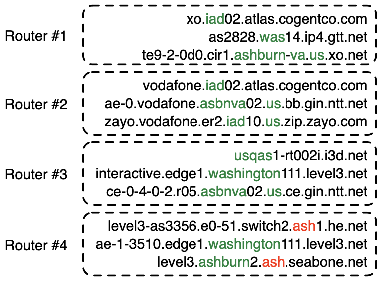
We inferred DNS-based geolocation heuristics using RTT measurements from 148 Ark VPs in 52 countries to constrain Hoiho, which automatically infers naming conventions in PTR records as regular expressions, and covered 819 different suffixes (e.g., ^.+\.([a-z]+)\d+\.level3\.net$ and ^.+\.([a-z]{3})\d+\.[a-z\d]+\.cogentco\.com$ extract geolocation hints in hostnames for Level3 and Cogent in the above figure). There is no dominant source of geohint observed in these naming conventions; 443 (54.1%) embedded IATA airport codes (e.g. IAD, WAS for the Washington D.C. area), 310 (37.9%) embedded place names (e.g. Ashburn for Ashburn, VA, US), 87 (10.6%) embedded the first six characters of a CLLI code (e.g. ASBNVA for Ashburn), and 12 (1.4%) embedded locodes (e.g. USQAS for Ashburn, VA, US). Interestingly, the operators that used CLLI and locodes had conventions that were more congruent with observed RTT values than operators that used IATA codes or place names. For the nodes in the ITDK, hoiho provided a geolocation inference for 127K, IXP provided a geolocation inference for 14K, and maxmind covered the remainder. The rules we inferred are usable via CAIDA’s Hoiho API.
ITDKs older than one year are publicly available, and ITDK 2024-02 is available to researchers and CAIDA members, after completing a simple form for access.
Acknowledgment: We are grateful to all of the Ark hosting sites, MaxMind’s freely available geolocation database, and academic research access to Iconectiv’s CLLI database to support this work.
In the first part of our blog series, we introduced our brand-new python module for scamper, the packet-prober underpinning much of Ark’s ongoing measurements. One aspect that we highlighted was the ability for potential users of Ark to develop their code locally, before running it on the Ark platform. When I develop measurement applications, I use a couple of local Raspberry Pis and my own workstation to get the code correct, and then copy the code to the CAIDA system to run the experiment using available Ark vantage points. The goal of this blog article is to describe different ways to locally develop your measurement experiment code.
Example #1: Starting small with one scamper process.
The easiest way to begin is with one scamper process running on the same system where you develop your python code. With scamper installed (we recommend that you use a package listed on the scamper website), start a scamper process, and make it available for measurement commands on a Unix domain socket. For example, you might run scamper as follows:
$ scamper -U /tmp/scamper -p 100
This will create a Unix domain socket to drive scamper at /tmp/scamper, and tell scamper that it can probe at up to 100 packets/second. You can adjust these parameters to what is appropriate locally.
You can then develop and debug your measurement code in Python. To use this scamper process, your Python code might begin as follows:
01 from scamper import ScamperCtrl

02

03 # use the scamper process available at /tmp/scamper

04 ctrl = ScamperCtrl(unix="/tmp/scamper")

05

06 # do a simple ping to 8.8.8.8 and print the outcome

07 o = ctrl.do_ping("8.8.8.8")

08 if o.min_rtt is not None:

09   print(f"{o.min_rtt.total_seconds()*1000):.1f} ms")

10 else:

11   print("no reply")
Example #2: Coordinating measurements among VPs.
Once you are comfortable using the python module with a single local scamper instance, you might want to test your code with multiple scamper instances, each representing a distinct vantage point. The scamper software includes the sc_remoted interface to support that. sc_remoted has features for authenticating endpoints with TLS, but you might choose to initially operate endpoints without the complexity of TLS.
sc_remoted listens on a port for inbound scamper connections, and makes Unix domain sockets — one for each VP — available in a nominated directory. The best idea is to create an empty directory for these sockets. You might run sc_remoted as follows:
$ mkdir -p /path/to/remote-sockets

$ sc_remoted -U /path/to/remote-sockets -P 50265
The first command creates the directory, because sc_remoted will not create that directory for you. The second command starts sc_remoted listening on port 50265 for incoming scamper connections, and will place Unix domain sockets in /path/to/remote-sockets as they arrive. Note, we use /path/to as a placeholder to the actual path in your local file system that is appropriate for your environment; you might put these sockets in a directory somewhere in your home directory, for example.
Then, on the systems that you want to act as vantage points, the following command:
$ scamper -p 100 -R 192.0.2.28:50265 -M foo.bar
will (1) start a scamper process, (2) tell it that it can probe at up to 100 packets-per-second, (3) connect it to the specified IP address and port to receive measurement commands from, and (4) tell it to identify itself as “foo.bar” to the remote controller. If you go into /path/to/remote-sockets, you might see the following:
$ cd /path/to/remote-sockets

$ ls -l

total 0

srwx------ 1 mjl mjl 0 Jan 22 16:57 foo.bar-192.0.2.120:12369
This socket represents the scamper process you just started. The filename begins with foo.bar, the parameter that you gave to scamper to identify itself. After the dash is the IP address and port number that the remote controller observed the remote system coming from. You can connect as many additional scamper instances as you like, and you will see them listed in the directory individually. You should name each differently with something meaningful to you (foo.bar, bar.baz, etc) so that you can identify them on the system on which you’re writing your python code.
The python code we wrote in Example #1 above might be modified as follows:
01 import sys

02 from scamper import ScamperCtrl

03

04 if len(sys.argv) != 2:

05   print("specify path to unix domain socket")

06   sys.exit(-1)

07

08 # use the remote scamper process available at the specified location

09 ctrl = ScamperCtrl(remote=sys.argv[1])

10

11 # do a simple ping to 8.8.8.8 and print the outcome

12 o = ctrl.do_ping("8.8.8.8")

13 if o.min_rtt is not None:

14   print(f"{o.min_rtt.total_seconds()*1000):.1f} ms")

15 else:

16   print("no reply")
And run as:
$ python ping.py /path/to/remote-sockets/foo.bar-192.0.2.120\:12369
If you have multiple remote-sockets in the directory, you can add them individually, or use all sockets in the directory. For example:
01 import sys

02 from datetime import timedelta

03 from scamper import ScamperCtrl

04

05 if len(sys.argv) != 3:

06   print("usage: single-radius.py $dir $ip")

07   sys.exit(-1)

08

09 ctrl = ScamperCtrl(remote_dir=sys.argv[1])

10 for i in ctrl.instances():

11   ctrl.do_ping(sys.argv[2], inst=i)

12

13 min_rtt = None

14 min_vp = None

15 for o in ctrl.responses(timeout=timedelta(seconds=10)):

16   if o.min_rtt is not None and (min_rtt is None or min_rtt > o.min_rtt):

17     min_rtt = o.min_rtt

18     min_vp = o.inst

19

20 if min_rtt is not None:

21   print(f"{min_vp.name} {(min_rtt.total_seconds()*1000):.1f} ms")

22 else:

23   print(f"no responses for {sys.argv[2]}")
and run this command:
$ python single-radius.py /path/to/remote-sockets 8.8.8.8
We encourage you to reach out via email if you have questions about using the module. In the first instance, you can email ark-info at caida.org.
ACM’s Internet Measurement Conference (IMC) is an annual highly selective venue for the presentation of Internet measurement and analysis research. The average acceptance rate for papers is around 25%. CAIDA researchers co-authored three papers and one poster that was be presented at the IMC conference in Montreal, Quebec on October 26 – 28, 2023. We link to these publications below.
On the Importance of Being an AS: An Approach to Country-Level AS Rankings
Bradley Huffaker, Alexander Marder, Romain Fontugne, kc claffy. ACM Internet Measurement Conference (IMC), 2023.
Recent geopolitical events demonstrate that control of Internet infrastructure in a region is critical to economic activity and defense against armed conflict. This geopolitical importance necessitates novel empirical techniques to assess which countries remain susceptible to degraded or severed Internet connectivity because they rely heavily on networks based in other nation states. Currently, two preeminent BGP-based methods exist to identify influential or market-dominant networks on a global scale-network-level customer cone size and path hegemony–but these metrics fail to capture regional or national differences.
We adapt the two global metrics to capture country-specific differences by restricting the input data for a country-specific metric to destination prefixes in that country. Although conceptually simple, our study required tackling methodological challenges common to most Internet measurement research today, such as geolocation, incomplete data, vantage point access, and lack of ground truth. Restricting public routing data to individual countries requires substantial downsampling compared to global analysis, and we analyze the impact of downsampling on the robustness and stability of our country-specific metrics. As a measure of validation, we apply our country-specific metrics to case studies of Australia, Japan, Russia, Taiwan, and the United States, illuminating aspects of concentration and interdependence in telecommunications markets. To support reproducibility, we will share our code, inferences, and data sets with other researchers.
IRRegularities in the Internet Routing Registry
Ben Du, Gautam Akiwate, Cecilia Testart, Alex C. Snoeren, kc claffy, Katherine Izhikevich, Sumanth Rao. ACM Internet Measurement Conference (IMC), 2023.
The Internet Routing Registry (IRR) is a set of distributed databases used by networks to register routing policy information and to validate messages received in the Border Gateway Protocol (BGP). First deployed in the 1990s, the IRR remains the most widely used database for routing security purposes, despite the existence of more recent and more secure alternatives. Yet, the IRR lacks a strict validation standard and the limited coordination across diferent database providers can lead to inaccuracies. Moreover, it has been reported that attackers have begun to register false records in the IRR to bypass operators’ defenses when launching attacks on the Internet routing system, such as BGP hijacks. In this paper, we provide a longitudinal analysis of the IRR over the span of 1.5 years. We develop a workflow to identify irregular IRR records that contain conflicting information compared to different routing data sources. We identify 34,199 irregular route objects out of 1,542,724 route objects from November 2021 to May 2023 in the largest IRR database and find 6,373 to be potentially suspicious.
Coarse-grained Inference of BGP Community Intent
Thomas Krenc, Alexander Marder, Matthew Luckie, kc claffy. ACM Internet Measurement Conference (IMC), 2023.
BGP communities allow operators to influence routing decisions made by other networks (action communities) and to annotate their network’s routing information with metadata such as where each route was learned or the relationship the network has with their neighbor (information communities). BGP communities also help researchers understand complex Internet routing behaviors. However, there is no standard convention for how operators assign community values, and significant efforts to scalably infer community meanings have ignored this high-level classification. We discovered that doing so comes at a significant cost in accuracy, of both inference and validation. To advance this narrow but powerful direction in Internet infrastructure research, we design and validate an algorithm to execute this first fundamental step: inferring whether a BGP community is action or information. We applied our method to 78,480 community values observed in public BGP data for May 2023. Validating our inferences (24,376 action and 54,104 informational communities) against available ground truth (6,259 communities) we find that our method classified 96.5% correctly. We found that the precision of a state-of-the-art location community inference method increased from 68.2% to 94.8% with our classifications. We publicly share our code, dictionaries, inferences, and datasets to enable the community to benefit from them.
CAIDA also contributed to one extended abstract:
Empirically Testing the PacketLab Model
Tzu-Bin Yan, Zesen Zhang, Bradley Huffaker, Ricky K. P. Mok, kc claffy, Kirill Levchenko. ACM Internet Measurement Conference (IMC) Poster, 2023.
PacketLab is a recently proposed model for accessing remote vantage points. The core design is for the vantage points to export low-level network operations that measurement researchers could rely on to construct more complex measurements. Motivating the model is the assumption that such an approach can overcome persistent challenges such as the operational cost and security concerns of vantage point sharing that researchers face in launching distributed active Internet measurement experiments. However, the limitations imposed by the core design merit a deeper analysis of the applicability of such model to real-world measurements of interest. We undertook this analysis based on a survey of recent Internet measurement studies, followed by an empirical comparison of PacketLab-based versus native implementations of common measurement methods. We showed that for several canonical measurement types common in past studies, PacketLab yielded similar results to native versions of the same measurements. Our results suggest that PacketLab could help reproduce or extend around 16.4% (28 out of 171) of all surveyed studies and accommodate a variety of measurements from latency, throughput, network path, to non-timing data.
A new working paper from the CAIDA GMI3S project summarizes key aspects of the European Union’s Digital Services Act (DSA), providing insight into how the EU plans to regulate large online platforms and services.
The DSA is intended to create a safer and more transparent online environment for consumers by imposing new obligations and accountability on companies like Meta, Google, Apple, and Amazon. The regulations target issues like illegal content, disinformation, political manipulation, and harmful algorithms. Systemic societal risks, like disinformation and political influence campaigns, are a major focus of the regulations.
Some key takeaways from the DSA overview:
The DSA signals that the EU is taking a hard line on enforcing accountability and responsible practices for dominant online platforms that have largely operated without oversight. The success of the regulations will depend on effective coordination and enforcement across the EU’s member states. However the Act provides a potential model for balancing innovation and consumer protection in the digital marketplace. Consumers may benefit from transparency and accountability of manipulative algorithms, more control over data, and protections against online harms.
Importantly, the data access mandate signals the EU’s commitment to leveraging academic expertise in shaping a healthier digital ecosystem. Researchers will be able to investigate systemic issues like algorithmic bias, political polarization, misinformation dynamics, and the mental health impacts of social media.
This DSA working paper provides valuable context on this ambitious attempt to regulate the digital economy.
To read further: